Dear ladies and gentleman,
I am an economist and new to modeling and programming. Please be forgiving with my lack of mathematical language.
I work on a simple non-linear trade model which derives prices and price changes, based on exogenous market shocks. For simplicity reasons right now the model only has two commodities (i) with no cross price elasticity and one region (j).
 Sets
         i  commodity    / cereals, rice /
         j  regions      / EUR / ;
The supply and demand functions are exponential.
supply(i,j)..  qs(i,j) =e= a(i,j)*(1+s_shift(i,j))*p(i)**es(i,j);
demand(i,j)..  qd(i,j) =e= b(i,j)*p(i)**ed(i,j);
a(i,j) calibration parameter supply function / givven
b(i,j) calibration parameter demand function / given
es(i,j) supply elasticities / given
ed(i,j) demand elasticities / given
s_shift(i,j) supply shift (%) / given
p(i) = price / positive variable
The goal function is to maximize producer (PS) and consumer surplus (CS), which is the integral between demand and supply curve.
objective..      goal =e= sum((i,j),PS(i,j)) + sum((i,j), CS(i,j));

prod_welf(i,j)..  PS(i,j) =e= qs(i,j)*p(i) - costs(i,j) ;
cons_welf(i,j)..  CS(i,j) =e= utility(i,j)- qd(i,j)*p(i) ;
cost_func(i,j)..  costs(i,j) =e= qs(i,j)*p(i) - a(i,j)/(es(i,j)+1)*(1+s_shift(i,j))*p(i)**(es(i,j)+1) ;
util_func(i,j)..  utility(i,j) =e= qd(i,j)*p(i) + b(i,j)/(ed(i,j)+1)*(pmax(i)**(ed(i,j)+1)- p(i)**(ed(i,j)+1));
After an exogenous production “shock” (shift of the supply curve) the nlp model finds a new market equilibrium (price and quantity). This works well.
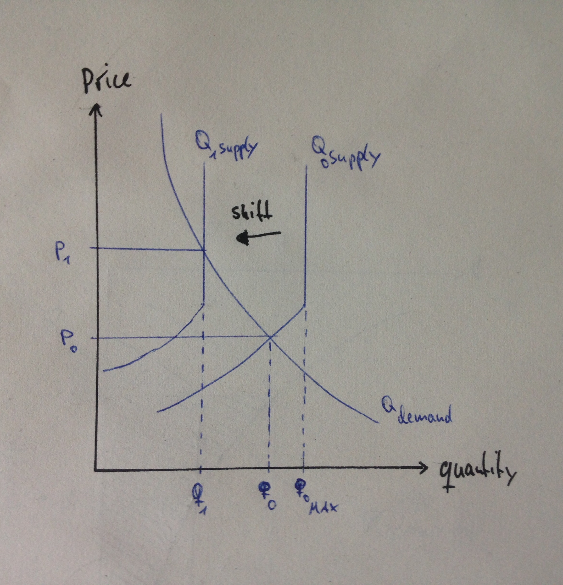
Now I want to implement and supply constraint. The supply function should be “cut” at a given quantity (picture 1: q0 max). No more than this maximum quantity could be supplied. If a shock hits the market, the cropped supply function is shifted (Q1 supply). The new maximum quantity that could be supplied can’t be bigger than “q0 max * (1 + s_shift)”. If this quantity constrains the solution then q1 = q0 max * (1 + s_shift).

Therefore I wrote a supply bound into the equations.
supply_bound(i,j).. qs(i,j) =l= qs0(i,j)*(1 + s_shift(i,j) + stock(i,j))
s_shift = supply shift
stock = additional storage capacity
qs0 * (1 + stock) = q0 max in picture 1
This supply_bound successfully limits the maximum quantity. But if the supply_bound constrains the solution space my model doesn’t find the right price (p1 in picture 1). It can not find a feasible solution anymore.
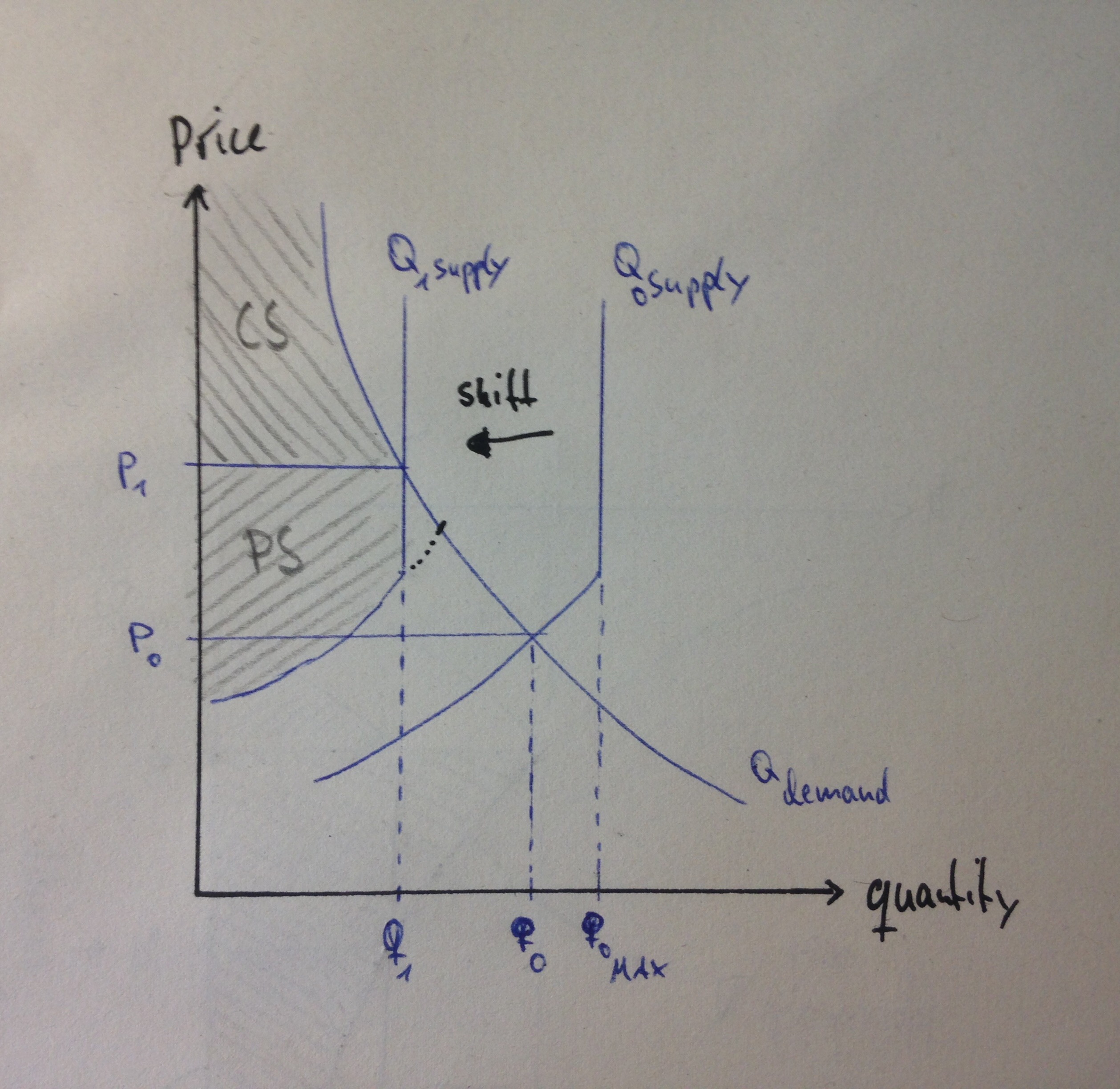
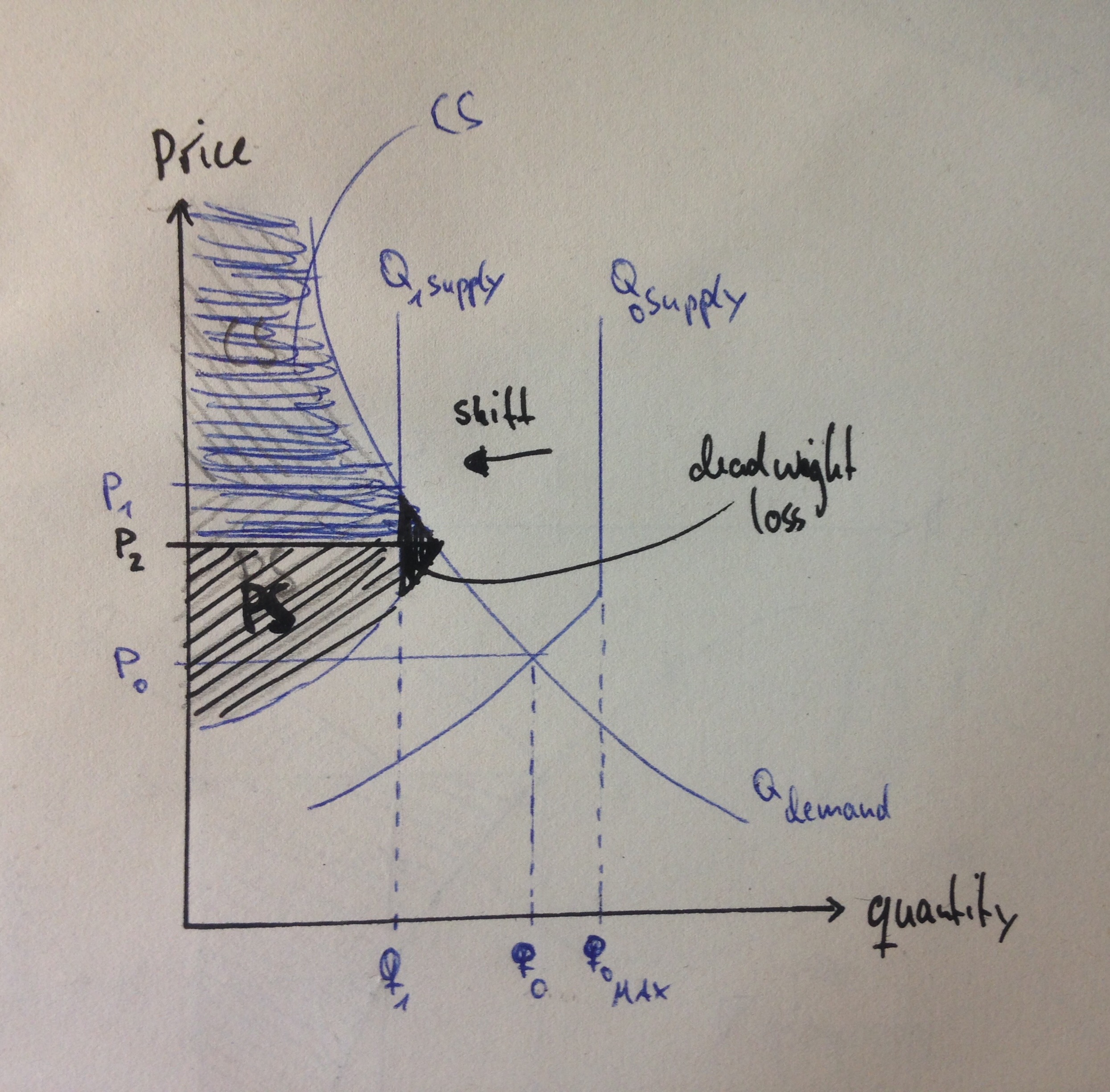
Right now the model does not calculate consumer and producer surplus right. Picture 2 shows the right solution. But my model cancels out the quantity (qd, qs) when consumer surplus and producer surplus is calculated. It comes out with the price p2 (picture 3 is integrated into the next post) and integrates the deadweight loss into his goal function. Mathematically this makes sense, because the area between the functions is bigger than in picture 2, but the implied quantity is outside of the solution space.

Is there a way implement different “sections” into one equation? E.g. between q = 0 and q < q max take this equation (q = a * p ^ es) with es = 0.3 and after q > q max (q = a * p ^ es) with es = 0.0001.
For q > q max the function would be almost vertical but the solver could still find a maximum. The price would increase drastically for q > q max while the quantity would only increase marginal.
If I could implement different “sections” into my supply equation, I maybe don’t need to change the goal function.
I attached the original GAMS code “simple trade model.gms”. A shock of minus 20% (s_shift = -0.2) to the initial supply of cereals (500 units) and no additional storage capacity (stock = 0) will result in a maximum supply quantity of 400 units. If I’m not wrong the right cereals price should be around 246. Instead the model does not change the price…
Thank you very much for your attention. Any hint or contribution is highly appreciated.
Cheers,
Hendrik
simple trade model.gms (4.38 KB)
