Model has been proven infeasible.

Hi,

I tried to solve my model for more than 3 months…
By reducing the variable, narrowing down the problem, and removing some complicated parts, the model already became a very all problem. However, the model still has been proven infeasible.

I tried to find the problem of infeasible in the equation, then I found it is not the problem because the guideline said it is infeasible for the starting part.
This model is a simple problem, it even can calculate by the hand(it is a calculation instead of the optimal problem)
I can calculate it by hands; however, I still do not know why it does not work
infeasible.docx (12.9 KB)
If anyone can help me, I will so appreciate it!!! Thank you so much!!!
image.png
Sincerely,
Sandy
image.png

You say

This model is a simple problem, it even can calculate by the hand(it is a calculation instead of the optimal problem)
I can calculate it by hands; however, I still do not know why it does not work

So why don’t you post this solution together with your model. I bet you it violates at least one of the following constraints E_DU(1), E_DU(2), E_DD2(2), E_DD2(3), E_DI(2), E_MU(3). Cplex IIS at least told me so.

BTW gms files can be easily attached in this forum, you don’t need to copy-paste GAMS code into a Word document. People don’t like to open Word documents from “strangers”.

-Michael

Hi Sandy

If you look at your model output, you will see the following message:

LP status(2): unbounded
Cplex Time: 0.00sec (det. 0.04 ticks)

The model has an unbounded ray.

If you search for the last line in this message, you will find:

Your model contains at least one variable with a coefficient in the objective but otherwise it does not show up in the constraint matrix (at least after preprocessing). The sign of the coefficient in the objective and the type of the variable (positive, negative, free) allows the model to become unbounded (or dual infeasible). Check the output for variables, which have a very large level, set a bound on the suspicious variables and see why it is not restricted by other parts of the model.

I looked at your model, and saw that all your variables are free, so the first thing I did (after a quick look at the model) is making them all positive variables (perhaps some of them can be negative, but that is for you to test).
The model then solves fine.

I hope this helps.
Cheers
Renger
PS. I replace the variable MIN with MINA as MIN is a function in Gams.

Hi!
Thank you for helping me.
I try to fix something and still get an infeasible result. Thus, I am wondering if the procedure I fixed it is correct.

set 
    t period /1*3/
    i parts /i1,i2/;

parameter
    MC capaciy/3000/
    DC capaciy/3000/
    AC capaciy/500/
    RC capaciy/500/
    a(i) number of part i in a product /i1 1, i2 4/
    c(i) Defected rate of part i /i1 0.8, i2 0.8/ 
    CR(t)'returned product shipped to CC at the beginning of period t'
    CU(t) 'reused product shipped to DC at the beginning of period t'
    CA(t) 'returned product shipped to A at the beginning of period t'
    X(t) /1 500, 2 1000/
    MF(t) /1 800, 2 1200/
    DF(t) /1 700, 2 1000/
    RQ /0/
    
    MPC production cost /30/
    DDC shipping cost /30/
    MOC ordering cost /30/
    MIC invenotry cost /20/
    MIPC product inventory cost /20/
    DIPC dc inventory cost /25/
    ;
Scalar
    d /0.3/ 
    b /0.2/ 
    z1/1.65/
    z2/1.65/ 
    ;
    
    CR(t)=b*X(t);
    CU(t+1)=d*CR(t);
    CA(t+1)=(1-d)*CR(t);
positive  variable
    MO(i,t) 'part i purchased from external at the beginning of period t'
    MP(t)   'product produced at mfg at the beginning of period t'
    DD(t)   'DC demand at the beginning of period t'
    MU(t)  'produce up to level at the beginning of period t'
    DU(t)  'order up to level at the beginning of period t';
free variable
    MIP(t)  'product inventory at mfg at the beginning of period t'
    DI(t)  'product inventory at DC at the beginning of period t'
    MI(i,t) 'part i inventory at mfg at the beginning of period t'
    z;
   
equation
    E_DU(t) 'order up to level at the beginning of period t'
    E_DD2(t)
    E_DI(t) 'product inventory at DC at the beginning of period t' 
    E_MU(t) 'produce up to level at the beginning of period t'
    E_MP(t) 'product produced at mfg at the beginning of period t'
    E_MIP(t) 'product inventory at mfg at the beginning of period t'
    E_MI(i,t) 'part i inventory at mfg at the beginning of period t'
    E_MO(i,t) 'part i purchased from external at the beginning of period t'
    E_DD(t) 'demand for DC'

    obj'objective function';
      
    E_DU(t)..DU(t+1)=E=DF(t+1)+z2*(DF(t)-X(t));
    E_DD2(t)..DD(t)=e=DU(t)-DI(t)-CU(t);
    E_DI(t)..DI(t+1)=e=DI(t)+(DD(t))+CU(t)-X(t);
    E_MU(t)..MU(t+1)=e=MF(t+1)+z1*(MF(t)-DD(t));
    E_MP(t)..MP(t)=e=MU(t+1)-MIP(t);
    E_MIP(t)..MIP(t+1)=e=MIP(t)+MP(t)-DD(t+1);
    E_MI(i,t)..MI(i,t+1)=e=MI(i,t)+MO(i,t)+RQ-a(i)*MP(t+1);
    E_MO(i,t)..MO(i,t+1)=e=a(i)* MP(t+1)- RQ-MI(i,t+1);
    E_DD(t)..DD(t+1)=l=DC-CU(t);
    
 
    MI.L("i1",t)=0;
    MI.L("i2",t)=0;
    MI.L("i1",t)=0;
    MI.L("i2",t)=0;

    MO.L("i1",t)=0;
    MO.L("i2",t)=0;

    DU.l(t)=0;
    MU.l(t)=0;

    MIP.l(t)=0;
    DI.l(t)=0;
    
    MP.up(t)=MC;
    
    obj..z=e=MIC*SUM(I,SUM(T,MI(i,t)))+MPC*SUM(t,MP(t))+DDC*SUM(t,DD(T))+MOC*SUM(I,SUM(T,MO(i,t)))+MIPC*SUM(t,MIP(T))+DIPC*SUM(t,DI(T))
;
    model LP/
    all/;
    Solve LP using LP minimizing z;
    Display MF,MU.L,MI.L,MI.L,MP.L,MIP.L,MO.L,DD.L,DU.L,DI.L,DF,X,CR,CU,CA;

the result is “Duplicate columns MO(i1.2) and MI(i1.2) make problem unbounded.”
MO(1,2)=a(1)* MP(2)- RQ-MI(1,2);
MI(1,2)=MI(1,1)+MO(1,1)+RQ-a(1)*MP(2);
If I do not consider MO’s and MI’s common variable (MP and RQ), we can see MO1,2 depending on MI1,2, and MI1,2 depending on MI1,1 and MO1,1. If MO1,1 and MI1,1 increase a lot, MI1,2 will increase a lot, and then MO1,2 will decrease unlimitedly. However, I set up MO as positive variable.

As I set up MO as a variable without the equal constraint and also give other variables for the model.

set 
    t period /1*3/
    i parts /i1,i2/;

parameter
    MC capaciy/3000/
    DC capaciy/3000/
    AC capaciy/500/
    RC capaciy/500/
    a(i) number of part i in a product /i1 1, i2 4/
    c(i) Defected rate of part i /i1 0.8, i2 0.8/ 
    CR(t)'returned product shipped to CC at the beginning of period t'
    CU(t) 'reused product shipped to DC at the beginning of period t'
    CA(t) 'returned product shipped to A at the beginning of period t'
    X(t) /1 500, 2 1000/
    MF(t) /1 800, 2 1200/
    DF(t) /1 700, 2 1000/
    RQ /0/
    
    MPC production cost /30/
    DDC shipping cost /30/
    MOC ordering cost /30/
    MIC invenotry cost /20/
    MIPC product inventory cost /20/
    DIPC dc inventory cost /25/
    ;
Scalar
    d /0.3/ 
    b /0.2/ 
    z1/1.65/
    z2/1.65/ 
    ;
    
    CR(t)=b*X(t);
    CU(t+1)=d*CR(t);
    CA(t+1)=(1-d)*CR(t);
positive  variable
    MO(i,t) 'part i purchased from external at the beginning of period t'
    MP(t)   'product produced at mfg at the beginning of period t'
    DD(t)   'DC demand at the beginning of period t'
    MU(t)  'produce up to level at the beginning of period t'
    DU(t)  'order up to level at the beginning of period t'
    QMD(t) 'actual shipping product from mfg to dc'
    QDC(t) 'actual shipping product from dc to customer'
    ;
free variable
    MIP(t)  'product inventory at mfg at the beginning of period t'
    DI(t)  'product inventory at DC at the beginning of period t'
    MI(i,t) 'part i inventory at mfg at the beginning of period t'
    z;
   
equation
    E_DU(t) 'order up to level at the beginning of period t'
    E_DD2(t)
    E_DI(t) 'product inventory at DC at the beginning of period t'
    C_QDC(t)
    C_QDC2(t)
    E_MU(t) 'produce up to level at the beginning of period t'
    E_MP(t) 'product produced at mfg at the beginning of period t'
    C_QMD(t)
    C_QMD2(t)
    E_MIP(t) 'product inventory at mfg at the beginning of period t'
    E_MI(i,t) 'part i inventory at mfg at the beginning of period t'
    E_MO(i,t)
    E_DD(t) 'demand for DC'
   

    obj'objective function';
      
    E_DU(t)..DU(t+1)=E=DF(t+1)+z2*(DF(t)-X(t));
    E_DD2(t)..DD(t)=e=DU(t)-DI(t)-CU(t);
    E_DI(t)..DI(t+1)=e=DI(t)+(QMD(t))+CU(t)-QDC(t+1);
    C_QDC(t)..QDC(t)=l=X(t+1);
    C_QDC2(t)..QDC(t+1)=l=DI(t+1)+QMD(t)+CU(t);
    E_MU(t)..MU(t+1)=e=MF(t+1)+z1*(MF(t)-DD(t));
    E_MP(t)..MP(t)=e=MU(t+1)-MIP(t);
    E_MIP(t)..MIP(t+1)=e=MIP(t)+MP(t)-QMD(t+1);
    C_QMD(t)..QMD(t)=l=DD(t+1)-CU(t);
    C_QMD2(t)..QMD(t+1)=l=MIP(t+1)+MP(t);
    E_MI(i,t)..MI(i,t+1)=e=MI(i,t)+MO(i,t)+RQ-a(i)*MP(t+1);
    E_MO(i,t)..MO(i,t+1)=e=a(i)* MP(t+1)- RQ-MI(i,t+1);
    E_DD(t)..DD(t+1)=l=DC-CU(t);

 
    MI.L("i1",t)=0;
    MI.L("i2",t)=0;
    MI.L("i1",t)=0;
    MI.L("i2",t)=0;
    MO.L("i1",t)=0;
    MO.L("i2",t)=0;

    DU.l(t)=0;
    MU.l(t)=0;

    MIP.l(t)=0;
    DI.l(t)=0;
    
    MP.up(t)=MC;
    
    obj..z=e=MIC*SUM(I,SUM(T,MI(i,t)))+MPC*SUM(t,MP(t))+DDC*SUM(t,DD(T))+MOC*SUM(I,SUM(T,MO(i,t)))+MIPC*SUM(t,MIP(T))+DIPC*SUM(t,DI(T))
;
    model LP/
    all/;
    Solve LP using LP minimizing z;
    Display MF,MU.L,MI.L,MI.L,MP.L,MIP.L,MO.L,DD.L,DU.L,DI.L,DF,X,CR,CU,CA;

the result is “Bound infeasibility column ‘QMD(2)’.”

There is the equation including QMD2
QMD2<=DD3-CU2
QMD2 <=MIP2+MP1
QMD2 is positive variable
MIP(2) =MIP(1)+MP(1)-QMD(2);
I am thinking if the problem is QMD2 be calculated as negative variable instead of positive. Hence, I change the constraint as
C_QDC(t)…QDC(t+1)=e=min(X(t+2),DI(t+1)+QMD(t)+CU(t));
C_QMD(t)…QMD(t+1)=e=min(DD(t+2)-CU(t+1),MIP(t+1)+MP(t));
And using Discontinuous Nonlinear Program to solve it. But the error still exists and become complicated (expectedly using DNLP instead of LP)
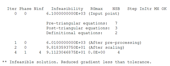
image.png
I am wondering if I utilized a reasonable method to debug the problem. Also, I would like to use LP to solve my question.
Any suggestions can help for me and I appreciate your help so much!

Sincerely,
Sandy

Hi,

I also have a question about using time series in the modeling and “.up” of variables.

set 
    t period /1*3/
    i parts /i1,i2/;

parameter
    MC capaciy/3000/
    DC capaciy/3000/
    AC capaciy/500/
    RC capaciy/500/
    a(i) number of part i in a product /i1 1, i2 4/
    c(i) Defected rate of part i /i1 0.8, i2 0.8/ 
    CR(t)'returned product shipped to CC at the beginning of period t'
    CU(t) 'reused product shipped to DC at the beginning of period t'
    CA(t) 'returned product shipped to A at the beginning of period t'
    X(t) /1 500, 2 1000/
    MF(t) /1 800, 2 1200/
    DF(t) /1 700, 2 1000/
    RQ /0/
    
    MPC production cost /30/
    DDC shipping cost /30/
    MOC ordering cost /30/
    MIC invenotry cost /20/
    MIPC product inventory cost /20/
    DIPC dc inventory cost /25/
    ;
Scalar
    d /0.3/ 
    b /0.2/ 
    z1/1.65/
    z2/1.65/ 
    ;
    
    CR(t)=b*X(t);
    CU(t+1)=d*CR(t);
    CA(t+1)=(1-d)*CR(t);
positive  variable
    MO(i,t) 'part i purchased from external at the beginning of period t'
    MP(t)   'product produced at mfg at the beginning of period t'
    DD(t)   'DC demand at the beginning of period t'
    MU(t)  'produce up to level at the beginning of period t'
    DU(t)  'order up to level at the beginning of period t'
    QMD(t) 'actual shipping product from mfg to dc'
    QDC(t) 'actual shipping product from dc to customer'
    ;
free variable
    MIP(t)  'product inventory at mfg at the beginning of period t'
    DI(t)  'product inventory at DC at the beginning of period t'
    MI(i,t) 'part i inventory at mfg at the beginning of period t'
    z;
   
equation
    E_DU(t) 'order up to level at the beginning of period t'
    E_DD2(t)
    E_DD(t) 'demand for DC'
    E_DI(t) 'product inventory at DC at the beginning of period t'
    C_QDC(t)
    C_QDC2(t)
    E_MU(t) 'produce up to level at the beginning of period t'
    E_MP(t) 'product produced at mfg at the beginning of period t'
    C_QMD(t)
    E_MIP(t) 'product inventory at mfg at the beginning of period t'
    E_MI(i,t) 'part i inventory at mfg at the beginning of period t'
    E_MO(i,t)
   

    obj'objective function';
      
    E_DU(t)..DU(t+1)=E=DF(t+1)+z2*(DF(t)-X(t));
    E_DD2(t)..DD(t)=l=DU(t)-DI(t)-CU(t);
    E_DD(t)..DD(t+1)=l=DC-CU(t);
    E_DI(t)..DI(t+1)=e=DI(t)+(QMD(t))+CU(t)-QDC(t+1);
    C_QDC(t)..QDC(t)=l=dd(t+1);
    C_QDC2(t)..QDC(t+1)=l=DI(t+1)+QMD(t)+CU(t);
    E_MU(t)..MU(t+1)=e=MF(t+1)+z1*(MF(t)-DD(t));
    E_MP(t)..MP(t)=e=MU(t+1)-MIP(t);
    E_MIP(t)..MIP(t+1)=e=MIP(t)+MP(t)-QMD(t+1);
    C_QMD(t)..QMD(t)=e=DD(t+1)-CU(t);
    E_MI(i,t)..MI(i,t+1)=e=MI(i,t)+MO(i,t)+RQ-a(i)*MP(t+1);
    E_MO(i,t)..MO(i,t+1)=e=a(i)* MP(t+1)- RQ-MI(i,t+1);


    MI.L("i1",t)=0;
    MI.L("i2",t)=0;
    MI.L("i1",t)=0;
    MI.L("i2",t)=0;
    MO.L("i1",t)=0;
    MO.L("i2",t)=0;

    DU.l(t)=0;
    MU.l(t)=0;

    MIP.l(t)=0;
    DI.l(t)=0;
    
    MP.up(t)=MC;
    QMD.up(t+1)=MIP.l(t+1)+MP.l(t);
    
    obj..z=e=MIC*SUM(I,SUM(T,MI(i,t)))+MPC*SUM(t,MP(t))+DDC*SUM(t,DD(T))+MOC*SUM(I,SUM(T,MO(i,t)))+MIPC*SUM(t,MIP(T))+DIPC*SUM(t,DI(T))
;
    model LP/
    all/;
    Solve LP using LP minimizing z;
    Display MF,MU.L,MI.L,MI.L,MP.L,MIP.L,MO.L,DD.L,DU.L,DI.L,DF,X,CR,CU,CA;

I change QMD(t+1)=l=MIP(t+1)+MP(t) to QMD.up(t+1)=MIP.l(t+1)+MP.l(t); I think they have the same definition. Is it correct?

  1. In this modeling, the result told me “Infeasibility row ‘C_QMD(3)’: 0 = -60.”
    As I saw the list, then it showed
    image.png
    I hope the equation for ‘C_QMD(3)’ likes other equations including DD(4); however, the set of t is from 1 to 3. It means the period here.
    The equation including lots of t+1 periods; however, I have no idea how to fix it. It is no okay for revising period form 1 to 4 because it will have the same problem for DD(5). Is there any way to stop the equation if the set range beyond the set I want?

Thank you so much!!!

Sincerely,
Sandy