"Model has been proven infeasible" error for two equations

halfa · March 19, 2025, 9:54am

Hello, I have written a code in the GAMS software that relates to AC power flow linear equations in electrical power engineering, but the output is not working correctly and gives the error “Model has been proven infeasible” due to equations eq1 and eq2. Is it possible to please review and guide me to resolve the issue?

Thank you in advance.

Sets
T /0*23/
B /B1*B5/
i "Buses" /1*33/
Slack(i) /1/;

Alias(i, j);

Sets Bus_B(B, i) "Mapping between B and Bus" / B1.6, B2.18, B3.21, B4.24, B5.30 /;

Scalar
cap_pv_max /20/,
cap_wt_max /3000/,
P_grid_MAX /2400/,
Q_grid_MAX /2000/,
phi_pv_wt /0.8/,
Prat_PV "KW" /800/,
f_dr /0.88/,
SunRadiation_STC /1000/,
Vin_W /0.5/,
Vrat_W /13/,
Vout_W /25/,
Prat_W "KW" /1000/,
SBase 'KVA'  /50000/;
**//////////////////**


Table E(t, b) "KW"
          B1            B2            B3            B4            B5
0         289.57        245.25        269.39        277.21        362.89
1         260.17        206.93        236.67        249.27        327.85
2         247.27        191.54        224.96        248.95        312.50
3         257.96        190.65        226.29        256.56        308.25
4         258.26        187.22        227.78        255.54        313.71
5         277.58        199.83        241.45        275.42        324.28
6         337.42        259.19        302.16        351.75        384.11
7         436.87        355.95        405.13        440.33        483.80
8         426.76        336.62        382.68        430.03        458.28
9         337.80        271.02        325.66        373.42        400.38
10        312.64        273.43        325.96        362.53        401.32
11        281.62        270.82        316.35        359.38        394.00
12        257.75        267.47        313.62        355.15        380.88
13        240.34        258.80        305.65        349.06        378.71
14        231.51        259.07        297.90        351.67        371.97
15        252.03        269.27        310.87        375.23        390.88
16        329.03        342.69        385.75        452.15        463.94
17        488.63        482.76        523.57        604.15        613.91
18        588.70        583.36        625.79        698.54        705.11
19        599.32        592.79        618.80        705.60        706.98
20        562.05        556.63        578.55        658.85        656.91
21        515.12        516.27        528.80        617.89        609.37
22        425.78        439.05        438.61        523.07        517.29
23        335.69        354.26        346.49        441.31        426.97;

Table SunRadiation(t, b) "W/m^2"
          B1         B2         B3         B4         B5
0         0          0          0          0          0
1         0          0          0          0          0
2         0          0          0          0          0
3         0          0          0          0          0
4         0          0          0          0          0
5         0          0          0          0          0
6         0          0          0          0          0
7         582        490        527        653        497
8         348        660        353        587        670
9         338        487        453        367        633
10        626        531        455        456        556
11        573        438        632        622        353
12        546        692        382        681        411
13        603        538        616        399        392
14        406        341        420        512        684
15        599        623        415        690        321
16        556        581        657        585        376
17        375        693        341        600        585
18        685        363        383        305        526
19        167        89         109        66         254
20        0          0          0          0          0
21        0          0          0          0          0
22        0          0          0          0          0
23        0          0          0          0          0;

Table WindSpeed(t, b) "m/s"
          B1        B2        B3        B4        B5
0         5         2         7         5         3
1         7         3         7         5         6
2         7         5         7         4         7
3         2         3         4         4         4
4         3         3         0         5         5
5         3         4         5         8         6
6         4         5         5         9         8
7         2         9         2         7         5
8         3         4         2         8         4
9         2         9         4         11        7
10        2         8         5         7         6
11        6         0         0         5         2
12        4         8         2         8         2
13        3         11        7         10        7
14        4         10        9         8         5
15        5         7         3         5         0
16        3         10        2         7         4
17        3         10        6         8         4
18        4         11        3         9         10
19        5         7         6         2         6
20        5         6         10        4         3
21        3         10        8         7         14
22        5         8         5         6         11
23        2         6         4         2         8;

Table LN(i, j, *)
             R             X             limit        G1           B1
1 .2         0.0922        0.047         3000         8.3334       -4.2481
2 .3         0.493         0.2511        3000         1.5590       -0.7941
3 .4         0.366         0.1864        3000         2.1001       -1.0696
4 .5         0.3811        0.1941        3000         2.0168       -1.0272
5 .6         0.819         0.707         3000         0.6772       -0.5846
6 .7         0.1872        0.6188        3000         0.4336       -1.4332
7 .8         1.7114        1.2351        3000         0.3719       -0.2684
8 .9         1.03          0.74          3000         0.6199       -0.4453
9 .10        1.044         0.74          3000         0.6171       -0.4374
10.11        0.1966        0.065         3000         4.4385       -1.4675
11.12        0.3744        0.1238        3000         2.3306       -0.7707
12.13        1.468         1.155         3000         0.4073       -0.3204
13.14        0.5416        0.7129        3000         0.6541       -0.8609
14.15        0.591         0.526         3000         0.9139       -0.8134
15.16        0.7463        0.545         3000         0.8459       -0.6178
16.17        1.289         1.721         3000         0.2699       -0.3603
17.18        0.732         0.574         3000         0.8189       -0.6421
2 .19        0.164         0.1565        3000         3.0893       -2.9480
19.20        1.5042        1.3554        3000         0.3552       -0.3200
20.21        0.4095        0.4784        3000         0.9996       -1.1678
21.22        0.7089        0.9373        3000         0.4969       -0.6570
3 .23        0.4512        0.3083        3000         1.4625       -0.9993
23.24        0.898         0.7091        3000         0.6640       -0.5243
24.25        0.896         0.7011        3000         0.6701       -0.5243
6 .26        0.203         0.1034        3000         3.7862       -1.9285
26.27        0.2842        0.1447        3000         2.7049       -1.3772
27.28        1.059         0.9337        3000         0.5143       -0.4534
28.29        0.8042        0.7006        3000         0.6843       -0.5962
29.30        0.5075        0.2585        3000         1.5145       -0.7714
30.31        0.9744        0.963         3000         0.5026       -0.4967
31.32        0.3105        0.3619        3000         1.3218       -1.5407
32.33        0.341         0.5302        3000         0.8306       -1.2915;

Table GenData(i, *) "KW and KVAR"
         Pmin        Pmax     Qmin       Qmax
6        0           3000     0          3000
18       0           3000     0          3000
21       0           3000     0          3000
24       0           3000     0          3000
30       0           3000     0          3000;

Table B_D(i, *) "KW and KVAR"
         Pd      Qd
1        0       0
2        100     60
3        90      40
4        120     80
5        60      30
6        60      20
7        200     100
8        200     100
9        60      20
10       60      20
11       45      30
12       60      35
13       60      35
14       120     80
15       60      10
16       60      20
17       60      20
18       90      40
19       90      40
20       90      40
21       90      40
22       90      40
23       90      50
24       420     200
25       420     200
26       60      25
27       60      25
28       60      20
29       120     70
30       200     600
31       150     70
32       210     100
33       60      40;

Parameters cx(i, j);

Variable obj, OPF_2D_P(i, j, t), OPF_2D_Q(i, j, t), Pg(t, i), Qg(t, i), P_demand(t, i), Q_demand(t, i),
         Pij(t, i, j), Qij(t, i, j), V(t, i), Vangle(t, i);

Equation obj_func, e_w1(t, b), e_w2(t, b), e_w3(t, b), e_w4(t, b), e_w5(t, b), e_pv(t, b), e_pv2(t, b), e_pv3(t, b),
         e_balance_P(t, b), e_balance_Q(t, b), e_g1(t, b), e_g2(t, b), e_g3(t, b), e_g4(t, b), e_g5(t, b),
         e_Pg(t, i), e_Qg(t, i), e_Pd(t, i), e_Qd(t, i), eq1, eq2, eq3, eq4, eq_OPF_2D_P, eq_OPF_2D_Q;

Positive Variable Ppv(t, b), Qpv(t, b), Pwind(t, b), Qwind(t, b), Qgrid(t, b), P_ex_pur(t, b), P_ex_sell(t, b);

Binary Variable K_pur(t, b), K_sell(t, b);

**PV Equation
e_pv(t, b)..  Ppv(t, b) =e= cap_pv_max*f_dr*(SunRadiation(t, b)/SunRadiation_STC);

e_pv2(t, b).. -Ppv(t, b)*tan(arccos(phi_pv_wt)) =l= Qpv(t, b);
e_pv3(t, b).. Qpv(t, b) =l= Ppv(t, b)*tan(arccos(phi_pv_wt));

**Wind Condition
e_w1(t, b)$(WindSpeed(t, b) < Vin_W or WindSpeed(t, b) > Vout_W).. Pwind(t, b) =e= 0;
e_w2(t, b)$(Vin_W <= WindSpeed(t, b) and WindSpeed(t, b) < Vrat_W).. Pwind(t, b) =e= cap_wt_max*(WindSpeed(t, b)-Vin_W)/(Vrat_W-Vin_W);
e_w3(t, b)$(Vrat_W <= WindSpeed(t, b) and WindSpeed(t, b) <= Vout_W).. Pwind(t, b) =e= cap_wt_max;

e_w4(t, b)..     -Pwind(t, b)*tan(arccos(phi_pv_wt)) =l= Qwind(t, b);
e_w5(t, b)..     Qwind(t, b) =l= Pwind(t, b)*tan(arccos(phi_pv_wt));

* GRID MODELING
e_g1(t, b)..     P_ex_pur(t, b) =l= P_grid_MAX*K_pur(t, b);
e_g2(t, b)..     P_ex_sell(t, b) =l= P_grid_MAX*K_sell(t, b);
e_g3(t, b)..     K_pur(t, b)+K_sell(t, b) =l= 1;

e_g4(t, b)..     -Q_grid_MAX =l= Qgrid(t, b);
e_g5(t, b)..     Qgrid(t, b) =l= Q_grid_MAX;

e_balance_P(t, b)..   Ppv(t, b)+Pwind(t, b)+P_ex_pur(t, b) =e= E(t, b)+P_ex_sell(t, b);
e_balance_Q(t, b)..   Qpv(t, b)+Qwind(t, b)+Qgrid(t, b) =e= E(t, b)*tan(arccos(phi_pv_wt));

* AC Power Flow
e_Pg(t, i)..   Pg(t, i) =e= sum(B$Bus_B(B, i), (Ppv(t, b)+Pwind(t, b)+P_ex_pur(t, b)-P_ex_sell(t, b))/Sbase);
e_Qg(t, i)..   Qg(t, i) =e= sum(B$Bus_B(B, i), (Qpv(t, b)+Qwind(t, b)+Qgrid(t, b))/Sbase);
* Aya in 2 moadele paein ham taghsim bar sbase mishavad?
e_Pd(t, i)..   P_demand(t, i) =e= B_D(i, 'Pd');
e_Qd(t, i)..   Q_demand(t, i) =e= B_D(i, 'Qd');

LN(i, j, 'X')$(LN(i, j, 'X')=0) = LN(j, i, 'X');
LN(i, j, 'R')$(LN(i, j, 'R')=0) = LN(j, i, 'R');
LN(i, j, 'B1')$(LN(i, j, 'B1')=0) = LN(j, i, 'B1');
LN(i, j, 'G1')$(LN(i, j, 'G1')=0) = LN(j, i, 'G1');
LN(i, j, 'Limit')$(LN(i, j, 'Limit')=0) =   LN(j, i, 'Limit');

cx(i, j)$(LN(i, j, 'limit') and LN(j, i, 'limit')) = 1;
cx(i, j)$(cx(j, i)) = 1;

Alias(i, i2);

Table WD(t,*)
        w                   d
*  t1   0                   1
   0   0.84                0.733473042484283
   1   0.0786666666666667  0.684511335492475
   2   0.0866666666666667  0.644122690036197
   3   0.117333333333333   0.6130691560297
   4   0.258666666666667   0.599733282530006
   5   0.361333333333333   0.588874071251667
   6   0.566666666666667   0.5980186702229
   7   0.650666666666667   0.626786054486569
   8   0.566666666666667   0.651743189178891
   9   0.484               0.706039245570585
   10  0.548               0.787007048961707
   11  0.757333333333333   0.839016955610593
   12  0.710666666666667   0.852733854067441
   13  0.870666666666667   0.870642027052772
   14  0.932               0.834254143646409
   15  0.966666666666667   0.816536483139646
   16  1                   0.819394170318156
   17  0.869333333333333   0.874071251666984
   18  0.665333333333333   1
   19  0.656               0.983615926843208
   20  0.561333333333333   0.936368832158506
   21  0.565333333333333   0.887597637645266
   22  0.556               0.809297008954087
   23  0.724               0.74585635359116;

eq_OPF_2D_P(i, j, t)$cx(i, j)..  OPF_2D_P(i, j, t) =e= (2*V(t, i)-1)*LN(i, j, 'G1')
                                 +sum(i2$(ord(i) ne ord(j)), LN(i, j, 'G1')*(V(t, i)+V(t, j)-1) + LN(i, j, 'B1')*(Vangle(t, i)-Vangle(t, j)));

eq_OPF_2D_Q(i, j, t)$cx(i, j)..  OPF_2D_Q(i, j, t) =e= -(2*V(t, i)-1)*LN(i, j, 'B1')
                                 +sum(i2$(ord(i) ne ord(j)), LN(i, j, 'B1')*(V(t, i)+V(t, j)-1) + LN(i, j, 'G1')*(Vangle(t, i)-Vangle(t, j)));

eq1(t, i)..   Pg(t, i) - WD(t,'d')*P_demand(t, i)/Sbase =e= sum(j$cx(j, i), OPF_2D_P(i, j, t));

eq2(t, i)..   Qg(t, i) - WD(t,'d')*Q_demand(t, i)/Sbase =e= sum(j$cx(j, i), OPF_2D_Q(i, j, t));

eq3(i, j, t)$cx(i, j)..   Pij(t, i, j) =e= ( LN(i, j, 'G1')*(V(t, i)-V(t, j)) ) + ( LN(i, j, 'B1')*(Vangle(t, i)-Vangle(t, j)) );
eq4(i, j, t)$cx(i, j)..   Qij(t, i, j) =e= ( -LN(i, j, 'B1')*(V(t, i)-V(t, j)) ) + ( LN(i, j, 'G1')*(Vangle(t, i)-Vangle(t, j)) );

V.lo(t, i)  = 0.95;
V.up(t, i)  = 1.05;
V.fx(t, slack)   = 1;

Vangle.up(t, i)     =  pi/2;
Vangle.lo(t, i)     = -pi/2;
Vangle.fx(t, slack)  = 0;

Pij.up(t, i, j)$((cx(i, j))) = 1*LN(i, j, 'Limit')/Sbase;
Pij.lo(t, i, j)$((cx(i, j))) =-1*LN(i, j, 'Limit')/Sbase;
Qij.up(t, i, j)$((cx(i, j))) = 1*LN(i, j, 'Limit')/Sbase;
Qij.lo(t, i, j)$((cx(i, j))) =-1*LN(i, j, 'Limit')/Sbase;

obj_func..   obj =e= 0;

Model mysystem /obj_func, e_w1, e_w2, e_w3, e_w4, e_w5, e_pv, e_pv2, e_pv3,
         e_balance_P, e_balance_Q, e_g5,
         e_Pg, e_Qg, e_Pd, e_Qd, eq1, eq2, eq3, eq4, eq_OPF_2D_P, eq_OPF_2D_Q/;

Option mip=cplex;

Solve mysystem min obj using mip;

Parameter report_Pg_Qg(t, i, *), report_V_Vangle(t, i, *);
report_Pg_Qg(t, i, 'Pg')   = Pg.l(t, i)*Sbase;
report_Pg_Qg(t, i, 'Qg')   = Qg.l(t, i)*Sbase;
report_V_Vangle(t, i, 'V')     = V.l(t, i);
report_V_Vangle(t, i, 'Angle') = Vangle.l(t, i);

Display Ppv.l, Qpv.l, Pwind.l, Qwind.l, P_ex_pur.l, P_ex_sell.l, Qgrid.l, Pg.l, Qg.l, Pij.l, Qij.l,
        report_Pg_Qg, report_V_Vangle, P_demand.l, Q_demand.l;

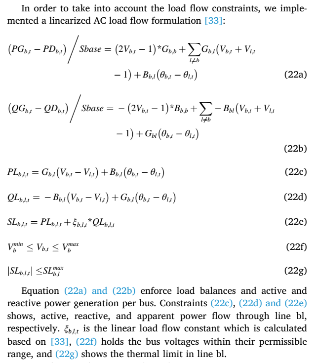
The linear equations from the image below were used:

halfa · March 22, 2025, 10:37am

@Fred_Fiand Hello sir, would it be possible for you to please give me some guidance?

Fred_Fiand · March 24, 2025, 7:54am

Hi @halfa ,

Cplex option IIS could be useful in this case. It producese the following output.

--- Conflict Refiner status (31): minimal conflict
--- Time spent on conflict find: 0.11 seconds

--- A conflict is a set of equations and variables (i.e. a submodel) which is 
--- infeasible but becomes feasible if any one equation or variable bound is dropped.
--- A problem may contain several independent conflicts but only one will be found per run.

Number of equations in conflict: 6
fixed: e_Pg(4,1) = 0
fixed: e_Pd(4,1) = 0
fixed: eq1(4,1) = 0
fixed: eq3(1,2,4) = 0
fixed: eq4(1,2,4) = 0
fixed: eq_OPF_2D_P(1,2,4) = -283.336

Number of variables in conflict: 3
fixed: V(4,1) = 1
upper: Pij(4,1,2) < 0.06
upper: Qij(4,1,2) < 0.06

I hope this helps!

Fred

halfa · March 25, 2025, 12:51am

@Fred_Fiand Thank you very much for your guidance. Should I add the iis to my code as follows?
option cplex_options = 'iis 1';

Fred_Fiand · March 25, 2025, 7:25am

No, you need to put it in a GAMS/Cplex Options file. See also here.

You could write that file on the fly as follows:

[...]
$onecho > cplex.opt
iis 1
$offEcho
mysystem.optfile = 1;

Solve mysystem min obj using mip;
[...]

I hope this helps!

halfa · March 25, 2025, 2:41pm

@Fred_Fiand Thank you very much. I removed the contents of the cplex.opt file and wrote only iis 1 and the output I received is as follows:

Time spent on conflict find =       0.36 seconds.
Minimal conflict found.

A conflict is a set equations and variables (ie a submodel) which is
infeasible but becomes feasible if any one equation or variable bound
is dropped.

A problem may contain several independent conflicts but only one will be
found per run.

Number of equations in the conflict:  7.
fixed: e_Qg(20,28) = 0
fixed: e_Qd(20,28) = 20
fixed: eq2(20,28) = 0
fixed: eq3(28,29,20) = 0
fixed: eq4(27,28,20) = 0
fixed: eq_OPF_2D_Q(28,27,20) = 14.5088
fixed: eq_OPF_2D_Q(28,29,20) = 19.0784

Number of variables in the conflict:  4.
lower: Pij(20,28,29) > -0.06
lower: Qij(20,27,28) > -0.06
lower: V(20,28) > 0.95
lower: V(20,29) > 0.95

This output is different from the output you provided. Can I implement the following codes in GAMS based on this output to resolve the issue? (If yes, can the equations that cause infeasibility also be corrected in this way?) Or should I consider another approach, such as correcting the input data?

Pij.fx('20','28','29') = -0.06;
Qij.fx('20','27','28') = -0.06;
V.fx('20','28') = 0.95;
V.fx('20','29') = 0.95;

Fred_Fiand · March 25, 2025, 3:28pm

No. The key is to understand first what the IIS actually is. From the documentation:

GAMS/Cplex also provides access to the Cplex Conflict Refiner previously known as IIS (Irreducibly Inconsistent Set). The conflict refinder takes an infeasible program and produces an set of conflicting constraints. Such a set consists of constraints and variable bounds which is infeasible but becomes feasible if any one member of the set is dropped. GAMS/Cplex reports the conflict in terms of GAMS equation and variable names and includes the conflict report as part of the normal solution listing.

Then you should ask yourself, how you ended up with such inconsistent constraints/bounds. Ist the model wrong? Is there a problem with the data? Or maybe both?

These are questions that usually can best be answered by the modeller.

I hope this helps!

halfa · March 25, 2025, 4:08pm

@Fred_Fiand Thank you for your time. Thanks.